Evaluation#
We stress that evaluation data must be different from training data, as neural networks have millions of parameters and can easily memorize thousands of samples. Avoid random train-test splits, try to create test datasets that mimic downstream tasks. If you are predicting among temporal surveys or across imaging platforms, your train-test data should reflect these partitions. Random sampling is almost never the right choice, biological data often has high spatial, temporal or taxonomic correlation that makes it easier for your model to generalize, but will fail when pushed into new situations.
DeepForest provides several evaluation metrics. There is no one-size-fits all evaluation approach, and the user needs to consider which evaluation metric best fits the task. There is significant information online about the evaluation of object detection networks. Our philosophy is to provide a user with a range of statistics and visualizations. Always visualize results and trust your judgment. Never be guided by a single metric.
Further Reading#
MeanAveragePrecision in torchmetrics
Average Intersection over Union#
DeepForest modules use torchmetric’s IntersectionOverUnion metric. This calculates the average overlap between predictions and ground truth boxes. This can be considered a general indicator of model performance but is not sufficient on its own for model evaluation. There are lots of reasons predictions might overlap with ground truth; for example, consider a model that covers an entire image with boxes. This would have a high IoU but a low value for model utility.
Mean-Average-Precision (mAP)#
mAP is the standard COCO evaluation metric and the most common for comparing computer vision models. It is useful as a summary statistic. However, it has several limitations for an ecological use case.
Not intuitive and difficult to translate to ecological applications. Read the sections above and visualize the mAP metric, which is essentially the area under the precision-recall curve at a range of IoU values.
The vast majority of biological applications use a fixed cutoff to determine an object of interest in an image. Perhaps in the future we will weight tree boxes by their confidence score, but currently we do things like, “All predictions > 0.4 score are considered positive detections”. This does not connect well with the mAP metric.
Precision and Recall at a set IoU threshold.#
This was the original DeepForest metric, set to an IoU of 0.4. This means that all predictions that overlap a ground truth box at IoU > 0.4 are true positives. As opposed to the torchmetrics above, it is intuitive and matches downstream ecological tasks. The drawback is that it is slow, coarse, and does not fully reward the model for having high confidence scores on true positives.
There is an additional difference between ecological object detection methods like tree crowns and traditional computer vision methods. Instead of a single or set of easily differentiated ground truths, we could have 60 or 70 objects that overlap in an image. How do you best assign each prediction to each ground truth?
DeepForest uses the hungarian matching algorithm to assign predictions to ground truth based on maximum IoU overlap. This is slow compared to the methods above, and so isn’t a good choice for running hundreds of times during model training see config[”validation”][”val_accuracy_interval”] for setting the frequency of the evaluate callback for this metric.
Calculating Evaluation Metrics#
Torchmetrics and loss scores#
These metrics are largely used during training to keep track of model performance. They are relatively fast and will be automatically run during training.
    m = main.deepforest()
    csv_file = get_data("OSBS_029.csv")
    root_dir = os.path.dirname(csv_file)
    m.config["validation"]["csv_file"] = csv_file
    m.config["validation"]["root_dir] = root_dir
    results = m.trainer.validate(m)
This creates a dictionary of the average IoU (’iou’) as well as ‘iou’ for each class. Here there is just one class, ‘Tree’. Then the COCO mAP scores. See Further Reading above for an explanation of mAP level scores. The val_bbox_regression is the loss function of the object detection box head, and the loss_classification is the loss function of the object classification head.
        classes                    0.0
           iou              0.6305446564807566
        iou/cl_0            0.6305446564807566
           map              0.04219449311494827
         map_50             0.11141198128461838
         map_75            0.025357535108923912
        map_large                  -1.0
       map_medium           0.05097917467355728
      map_per_class                -1.0
        map_small                   0.0
          mar_1            0.008860759437084198
         mar_10             0.03417721390724182
         mar_100            0.08481013029813766
    mar_100_per_class              -1.0
        mar_large                  -1.0
       mar_medium           0.09436620026826859
        mar_small                   0.0
   val_bbox_regression      0.5196723341941833
   val_classification       0.4998389184474945
Advanced tip: Users can set the frequency of pytorch lightning evaluation using kwargs passed to main.deepforest.create_trainer(). For example check_val_every_n_epochs.
Recall and Precision at a fixed IoU Score#
To get a recall and precision at a set IoU evaluation score, specify an annotations’ file using the m.evaluate method.
m = main.deepforest()
csv_file = get_data("OSBS_029.csv")
root_dir = os.path.dirname(csv_file)
results = m.evaluate(csv_file, root_dir, iou_threshold = 0.4)
The returned object is a dictionary containing the three keys: results, recall, and precision. The result key in the csv-file represents the intersection-over-union score for each ground truth object.
results["results"].head()
    prediction_id  truth_id      IoU    image_path  match
39             39         0  0.00000  OSBS_029.tif  False
19             19         1  0.50524  OSBS_029.tif   True
44             44         2  0.42246  OSBS_029.tif   True
67             67         3  0.41404  OSBS_029.tif   True
28             28         4  0.37461  OSBS_029.tif  False
This dataframe contains a numeric id for each predicted crown in each image and the matched ground truth crown in each image. The intersection-over-union score between predicted and ground truth (IoU), and whether that score is greater than the IoU threshold (’match’).
The recall is the proportion of ground truth that has a true positive match with a prediction based on the intersection-over-union threshold. The default threshold is 0.4 and can be changed in the model.evaluate(iou_threshold=<>)
results["box_recall"]
0.705
The regression box precision is the proportion of predicted boxes which overlap a ground truth box.
results["box_precision"]
0.781
Worked example of calculating IoU and recall/precision values#
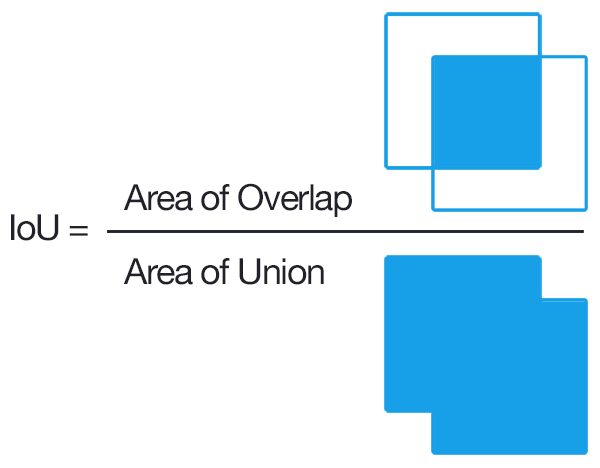
To convert overlap among predicted and ground truth bounding boxes into measures of accuracy and precision, the most common approach is to compare the overlap using the intersection-over-union metric (IoU). IoU is the ratio between the area of the overlap between the predicted polygon box and the ground truth polygon box divided by the area of the combined bounding box region.
Let’s start by getting some sample data and predictions
from deepforest import evaluate
from deepforest import main
from deepforest import get_data
from deepforest import visualize
import os
import pandas as pd

m = main.deepforest()
m.use_release()

csv_file = get_data("OSBS_029.csv")
predictions = m.predict_file(csv_file=csv_file, root_dir=os.path.dirname(csv_file))
predictions.head()
    xmin   ymin   xmax   ymax label     score    image_path
0  330.0  342.0  373.0  391.0  Tree  0.802979  OSBS_029.tif
1  216.0  206.0  248.0  242.0  Tree  0.778803  OSBS_029.tif
2  325.0   44.0  363.0   82.0  Tree  0.751573  OSBS_029.tif
3  261.0  238.0  296.0  276.0  Tree  0.748605  OSBS_029.tif
4  173.0    0.0  229.0   33.0  Tree  0.738209  OSBS_029.tif
ground_truth = pd.read_csv(csv_file)
ground_truth.head()
     image_path  xmin  ymin  xmax  ymax label
0  OSBS_029.tif   203    67   227    90  Tree
1  OSBS_029.tif   256    99   288   140  Tree
2  OSBS_029.tif   166   253   225   304  Tree
3  OSBS_029.tif   365     2   400    27  Tree
4  OSBS_029.tif   312    13   349    47  Tree
visualize.plot_prediction_dataframe(predictions, ground_truth, root_dir = os.path.dirname(csv_file))
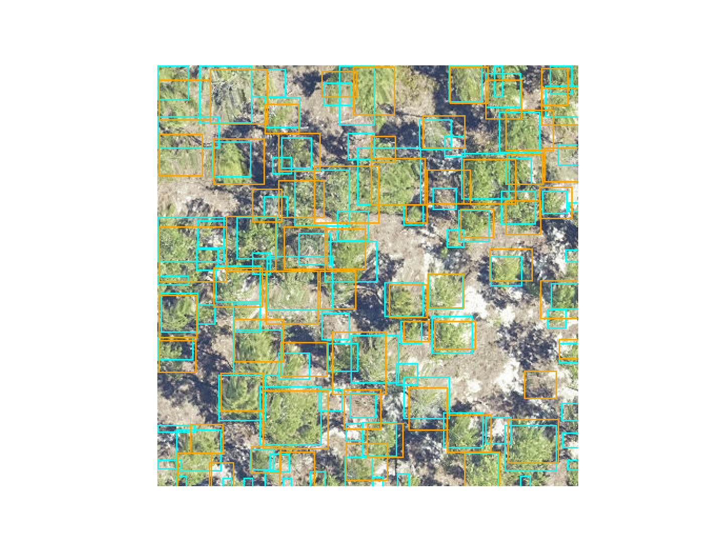
The IoU metric ranges between 0 (no overlap) to 1 (perfect overlap). In the wider computer vision literature, the conventional threshold value for overlap is 0.5, but this value is arbitrary and does not ultimately relate to any particular ecological question. We considered boxes which have an IoU score of greater than 0.4 as true positive, and scores less than 0.4 as false negatives. The 0.4 value was chosen based on visual evaluation of the threshold that indicated a good visual match between the predicted and observed crown. We tested a range of overlap thresholds from 0.3 (less overlap among matching crowns) to 0.6 (more overlap among matching crowns) and found that 0.4 balanced a rigorous cutoff without spuriously removing trees that would be useful for downstream analysis.
After computing the IoU for the ground truth data, we get the resulting dataframe.
result = evaluate.evaluate_image(predictions=predictions, ground_df=ground_truth, root_dir=os.path.dirname(csv_file), savedir=None)
result.head()
    prediction_id  truth_id       IoU predicted_label true_label
90             90         0  0.059406            Tree       Tree
65             65         1  0.335366            Tree       Tree
17             17         2  0.578551            Tree       Tree
50             50         3  0.532902            Tree       Tree
34             34         4  0.595862            Tree       Tree
Where prediction_id is a unique ID to each predicted tree box. truth is a unique ID to each ground truth box. The predicted and true labels are tree in this, case but could generalize to multi-class problems. From here we can calculate precision and recall at a given IoU metric.
result["match"] = result.IoU > 0.4
true_positive = sum(result["match"])
recall = true_positive / result.shape[0]
precision = true_positive / predictions.shape[0]
recall
0.819672131147541
precision
0.5494505494505495
This can be stated as 81.97% of the ground truth boxes are correctly matched to a predicted box at IoU threshold of 0.4, and 54.94% of predicted boxes match a ground truth box. Optimally we want a model that is both precise and accurate.
The above logic is wrapped into the evaluate.evaluate() function
result = evaluate.evaluate(predictions=predictions, ground_df=ground_truth,root_dir=os.path.dirname(csv_file), savedir=None)
This is a dictionary with keys
result.keys()
dict_keys(['results', 'box_precision', 'box_recall', 'class_recall'])
The added class_recall dataframe is mostly relevant for multi-class problems, in which the recall and precision per class is given.
result["class_recall"]
  label  recall  precision  size
0  Tree     1.0    0.67033    61
How to average evaluation metrics across images?#
One important decision was how to average precision and recall across multiple images. Two reasonable options might be to take all predictions and all ground truth and compute the statistic on the entire dataset. This strategy makes more sense for evaluation data that is relatively homogenous across images. We prefer to take the average of per-image precision and recall. This helps balance the dataset if some images have many objects and others have few objects, such as when you are comparing multiple habitat types. Users are welcome to calculate their own statistics directly from the results dataframe.
result["results"].head()
    prediction_id  truth_id       IoU  ... true_label    image_path  match
90             90         0  0.059406  ...       Tree  OSBS_029.tif  False
65             65         1  0.335366  ...       Tree  OSBS_029.tif  False
17             17         2  0.578551  ...       Tree  OSBS_029.tif   True
50             50         3  0.532902  ...       Tree  OSBS_029.tif   True
34             34         4  0.595862  ...       Tree  OSBS_029.tif   True
Evaluating tiles too large for memory#
The evaluation method uses deepforest.predict_image for each of the paths supplied in the image_path column. This means that the entire image is passed for prediction. This will not work for large images. The deepforest.predict_tile method does a couple things under the hood that need to be repeated for evaluation.
psuedo_code:
output_annotations = deepforest.preprocess.split_raster(
    path_to_raster = <path>,
    annotations_file = <original_annotation_path>,
    base_dir = <location to save crops>
    patch_size = <size of each crop>

)

output_annotations.to_csv("new_annotations.csv")

results = model.evaluate(
    csv_file="new_annotations.csv",
    root_dir=<base_dir from above>
)