Getting started#

Demo#

How do I use a pretrained model to predict an image?#

from deepforest import main
from deepforest import get_data
import matplotlib.pyplot as plt

model = main.deepforest()
model.use_release()

sample_image_path = get_data("OSBS_029.png")
img = model.predict_image(path=sample_image_path, return_plot=True)

#predict_image returns plot in BlueGreenRed (opencv style), but matplotlib likes RedGreenBlue, switch the channel order. Many functions in deepforest will automatically perform this flip for you and give a warning.
plt.imshow(img[:,:,::-1])

_images/getting_started1.png

** please note that this video was made before the deepforest-pytorch -> deepforest name change. **

For single images, predict_image can read an image from memory or file and return predicted tree bounding boxes.

Sample data#

DeepForest comes with a small set of sample data that can be used to test out the provided examples. The data resides in the DeepForest data directory. Use the get_data helper function to locate the path to this directory, if needed.

sample_image = get_data("OSBS_029.png")
sample_image
'/Users/benweinstein/Documents/DeepForest/deepforest/data/OSBS_029.png'

To use images other than those in the sample data directory, provide the full path for the images.

image_path = get_data("OSBS_029.png")
boxes = model.predict_image(path=image_path, return_plot = False)

boxes.head()
         xmin        ymin        xmax        ymax  label    scores
334.708405  342.333954  375.941376  392.187531      0  0.736650
295.990601  371.456604  331.521240  400.000000      0  0.714327
216.828201  207.996216  245.123276  240.167023      0  0.691064
276.206848  330.758636  303.309631  363.038422      0  0.690987
328.604736   45.947182  361.095276   80.635254      0  0.638212

For the release model, there is only one category “Tree”, which is numeric 0 label.

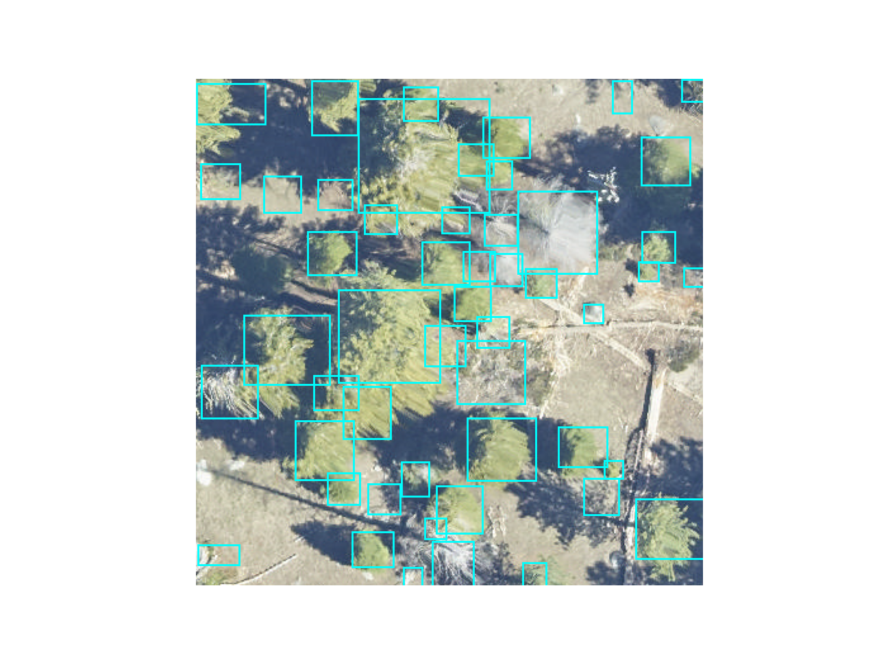
Predict a tile#

Large tiles covering wide geographic extents cannot fit into memory during prediction and would yield poor results due to the density of bounding boxes. Often provided as geospatial .tif files, remote sensing data is best suited for the predict_tile function, which splits the tile into overlapping windows, performs prediction on each of the windows, and then reassembles the resulting annotations.

Let’s show an example with a small image. For larger images, patch_size should be increased.

raster_path = get_data("OSBS_029.tif")
# Window size of 300px with an overlap of 25% among windows for this small tile.
predicted_raster = model.predict_tile(raster_path, return_plot = True, patch_size=300,patch_overlap=0.25)

# View boxes overlayed when return_plot=True, when False, boxes are returned.
plt.imshow(predicted_raster)
plt.show()

** Please note the predict tile function is sensitive to patch_size, especially when using the prebuilt model on new data**

We encourage users to try out a variety of patch sizes. For 0.1m data, 400-800px per window is appropriate, but it will depend on the density of tree plots. For coarser resolution tiles, >800px patch sizes have been effective, but we welcome feedback from users using a variety of spatial resolutions.

Predict a set of annotations#

During evaluation of ground truth data, it is useful to have a way to predict a set of images and combine them into a single data frame. The predict_generator method allows a user to point towards a file of annotations and returns the predictions for all images.

Consider a headerless annotations.csv file in the following format

image_path, xmin, ymin, xmax, ymax, label

with each bounding box on a separate row. The image path is relative to the root dir. Its often easiest to just save the .csv file alongside the images.

We can view predictions by supplying a save dir (”.” = current directory). Predictions in green, annotations in black.

import os

csv_file = get_data("testfile_deepforest.csv")
boxes = model.predict_file(csv_file=csv_file, root_dir = os.path.dirname(csv_file),savedir=".")

Projecting predictions#

DeepForest operates on image data without any concept of geopgraphic projection. Annotations and predictions are made in reference to the image coordinate system (0,0). It is often useful to transform this to geographic coordinates. Rasterio provides us with helpful utilities to do this based on a projected image.

For example, consider some sample data that comes with package. We can read in the image, get the transform and coordinate reference system (crs).

    img = get_data("OSBS_029.tif")
    r = rasterio.open(img)
    transform = r.transform 
    crs = r.crs
    print(crs)

    CRS.from_epsg(32617)

We can predict tree crowns in the image and then convert them back into projected space

    m = main.deepforest()
    m.use_release(check_release=False)
    df = m.predict_image(path=img)
    gdf = utilities.annotations_to_shapefile(df, transform=transform, crs=crs)

    gdf.total_bounds
    array([ 404211.95, 3285102.85,  404251.95, 3285142.85])
    gdf.crs
    <Projected CRS: EPSG:32617>
    Name: WGS 84 / UTM zone 17N
    Axis Info [cartesian]:
    - [east]: Easting (metre)
    - [north]: Northing (metre)
    Area of Use:
    - undefined
    Coordinate Operation:
    - name: UTM zone 17N
    - method: Transverse Mercator
    Datum: World Geodetic System 1984
    - Ellipsoid: WGS 84
    - Prime Meridian: Greenwich

Customizing box appearance for predictions#

The color and line thickness of boxes can be customized using the color and thickness arguments. color is the color of the bounding box as a tuple of BGR color, e.g. orange annotations is (0, 165, 255). thickness is the thickness of the rectangle border line in pixels.

image_path = get_data("OSBS_029.png")
boxes = model.predict_image(path=image_path, return_plot = True, color=(0, 165, 255), thickness=3)